Computer modeling

The ping-pong balls avalanche system is a granular flow (the ping-pong balls) interacting strongly with a fluid flow (the air). By strongly interacting we mean that any accurate description must include the force of the air on the balls and the force of the balls on the air.

This system is described by well known equations: The air flow obeys the Navier-Stokes equations, and each ping-pong ball follows Newtons law. The force on each ball contains contributions from gravity, ball-ball forces, ball-ground forces and air-drag forces. The air-drag force comes from the no-slip boundary condition between the balls and the air flow. The large range of length and time scales makes direct integration of the equations of motion very difficult. Ball-ball collisions occur over time intervals of order $10^{-4}\mbox{s}$ whereas the duration of the flow is around $30\mbox{s}$. To resolve the collisions time steps at least ten times smaller must be used, thus 10 million or so time steps are necessary. The length scales in the problem are the length of the ski jump $O(100m)$, the length scale given by the volume of the flow $O(1\mbox{m})$, the size of the balls themselves $O(0.01m)$ and the air flow details around the balls $O(0.001\mbox{m})$. A direct integration would require a grid of size $100\times10\times10/0.001^3=10^{13}$. Direct calculations require at least order $10^{20}$ operations and are obviously infeasible.

The most important simplification to make is in the interaction between the balls and the air. If we consider the air flow only on a scale much larger than the individual ping-pong balls we can replace the air-ball no-slip boundary condition by an empirical body force representing the average drag of the balls on the air. If the grid squares are taken as $1\mbox{m}$ then the total grid size is reduced to $10^4$ and the problem becomes feasible. The volume concentration of the balls is accounted for as an additional term in the conservation of mass equation. As a first approximation we regard the flow as inviscid since the Reynolds number for the flow is of order $10^3$ (based on the smallest length scale, ball diameter, and ball terminal velocity) and the drag forces are included explicitly. This approach fails if there is separation in the flow field. Although the Reynolds number for the whole flow is of order $10^6$, the flow shape is streamlined and the volume density of the balls is low so separation may not occur. This is a standard approximation in the theory of streamlined bodies. Since the Mach numbers in the flow are low we assume the density of the air is constant. There are no satisfactory continuum theories for granular flows -- attempts to extend the kinetic theory of granular matter to dense flows have not been successful -- so a direct approach is necessary where the equation of motion for each ball are integrated. This is feasible for systems of several million balls on current supercomputers.

We choose a simple model for ball-ball and ball-ground interactions. We assume that the normal force $N$ is given by a damped spring and that the tangential force is given by Coulomb friction. The friction force is thus $\mu N$ opposing the direction of slip, or $0$ when there is no slip. This form of friction law is not accurate for long lasting contacts. A more realistic friction law requires that the friction can take all values between $-\mu N$ and $+\mu N$ depending on the history of the contact and thus requires extra variables to describe the history of the contact. During the flow the the volume densities are low, thus the contact times between balls will be small so the complexity of accurately modeling static force distributions is unnecessary for these flows.

We scale the air pressure by the air density and eliminate gravity by adding a static potential, $\textbf{x}\cdot\textbf{g}$, to the pressure. Since we envisage solving the fluid flow equations over a scale larger than ball diameter there is no direct coupling between air pressure changes and air shear rates and the balls. Coupling between the balls' angular velocity and the air is also neglected. The direct effect of the static air pressure on the balls is accounted for by adjusting the gravitational force acting on the balls.

The system obeys the following equations for conservation of volume, mass and momentum

$md^2/4 \ddot \mathbf{w}_i = -\textbf{r}_{ij} \wedge (\textbf{f}_{ij} + \textbf{h}_i )$	volume identity
$md^2/4 \ddot \mathbf{w}_i = -\textbf{r}_{ij} \wedge (\textbf{f}_{ij} + \textbf{h}_i )$	mass conservation
$md^2/4 \ddot \mathbf{w}_i = -\textbf{r}_{ij} \wedge (\textbf{f}_{ij} + \textbf{h}_i )$	air momentum conservation
$md^2/4 \ddot \mathbf{w}_i = -\textbf{r}_{ij} \wedge (\textbf{f}_{ij} + \textbf{h}_i )$	ball $i$ momentum conservation
$md^2/4 \ddot \mathbf{w}_i = -\textbf{r}_{ij} \wedge (\textbf{f}_{ij} + \textbf{h}_i )$	ball $i$ angular momentum conservation

The independent variables are the following:

$\mathbf{w}_i$	volume density of air
$\mathbf{w}_i$	air velocity
$\mathbf{w}_i$	air pressure
$\mathbf{w}_i$	position of ball $i$
$\mathbf{w}_i$	velocity of ball $i$
$\mathbf{w}_i$	angular velocity of ball $i$

The auxillary variables are the following:

$\textbf{h}_i = 1_{r_{gi}<d/2} (\hat \textbf{r}_{gi} + \mu_g \hat \textbf{t}_{gi}) [k_g (d/2-r_{gi}) + \eta_g \hat \textbf{r}_{gi} \cdot \textbf{u}_{gi}]$	volume density of balls
$\textbf{h}_i = 1_{r_{gi}<d/2} (\hat \textbf{r}_{gi} + \mu_g \hat \textbf{t}_{gi}) [k_g (d/2-r_{gi}) + \eta_g \hat \textbf{r}_{gi} \cdot \textbf{u}_{gi}]$	total drag
$\textbf{h}_i = 1_{r_{gi}<d/2} (\hat \textbf{r}_{gi} + \mu_g \hat \textbf{t}_{gi}) [k_g (d/2-r_{gi}) + \eta_g \hat \textbf{r}_{gi} \cdot \textbf{u}_{gi}]$	drag on ball $i$
$\textbf{h}_i = 1_{r_{gi}<d/2} (\hat \textbf{r}_{gi} + \mu_g \hat \textbf{t}_{gi}) [k_g (d/2-r_{gi}) + \eta_g \hat \textbf{r}_{gi} \cdot \textbf{u}_{gi}]$	drag coefficient
$\textbf{h}_i = 1_{r_{gi}<d/2} (\hat \textbf{r}_{gi} + \mu_g \hat \textbf{t}_{gi}) [k_g (d/2-r_{gi}) + \eta_g \hat \textbf{r}_{gi} \cdot \textbf{u}_{gi}]$	ball-ball force
$\textbf{h}_i = 1_{r_{gi}<d/2} (\hat \textbf{r}_{gi} + \mu_g \hat \textbf{t}_{gi}) [k_g (d/2-r_{gi}) + \eta_g \hat \textbf{r}_{gi} \cdot \textbf{u}_{gi}]$	ball-ground force

where $\textbf{u}_{Ri} = \textbf{u}_i-\textbf{u}_a$ is the relative velocity between air and ball $i$
$\textbf{r}_{ij} = (\textbf{r}_i-\textbf{r}_j)/2$ is the vector to the contact point, $\textbf{u}_{ij} = \textbf{u}_i-\textbf{u}_j -\hat\textbf{r}_{ij}\wedge (\mathbf{w}_i+\mathbf{w}_j)$ is the ball-ball relative velocity, $\textbf{t}_{ij} = \textbf{u}_{ij} -\hat \textbf{r}_{ij}(\hat \textbf{r}_{ij}\cdot \textbf{u}_{ij})$ is the ball-ball tangential velocity. $\textbf{r}_{gi}$, $\textbf{u}_{gi}$ and $\textbf{t}_{gi}$ are similarly defined for ball-ground collisions.

Standard vector calculus notation is used where $\vert.\vert$ denotes the norm and $\hat.$ a unit vector. Thus for a vector $\textbf{v}$

$$v = \vert\textbf{v}\vert$$ (1)

$$\hat \textbf{v} = \left\{ \begin{array}{ll} \textbf{v}/\vert\textbf{v}\vert & \vert\textbf{v}\vert > 0 \\ \textbf{0} & \vert\textbf{v}\vert = 0. \end{array}\right.$$ (2)

The indicator function is defined for an inequality $R$ by

$$1_R = \left\{\begin{array}{ll} 1 & \mbox{if $R$} \\ 0 & \mbox{if not $R$}. \end{array}\right.$$ (3)

The main parameters (at standard temperature and pressure) are the following:

$9.81\,\mbox{ms}^{-2}$	$9.81\,\mbox{ms}^{-2}$	description
$9.81\,\mbox{ms}^{-2}$	$9.81\,\mbox{ms}^{-2}$	mass
$9.81\,\mbox{ms}^{-2}$	$9.81\,\mbox{ms}^{-2}$	ball diameter
$9.81\,\mbox{ms}^{-2}$	$9.81\,\mbox{ms}^{-2}$	ball stiffness
$9.81\,\mbox{ms}^{-2}$	$9.81\,\mbox{ms}^{-2}$	ball-ball restitution
$9.81\,\mbox{ms}^{-2}$	$9.81\,\mbox{ms}^{-2}$	ball-ball friction
$9.81\,\mbox{ms}^{-2}$	$9.81\,\mbox{ms}^{-2}$	ball-ground restitution
$9.81\,\mbox{ms}^{-2}$	$9.81\,\mbox{ms}^{-2}$	ball-ground friction
$9.81\,\mbox{ms}^{-2}$	$9.81\,\mbox{ms}^{-2}$	air density
$9.81\,\mbox{ms}^{-2}$	$9.81\,\mbox{ms}^{-2}$	kinematic air viscosity
$9.81\,\mbox{ms}^{-2}$	$9.81\,\mbox{ms}^{-2}$	gravity

The auxillary parameters are the following:

$\eta_g = -2\sqrt{km}/\sqrt{1+(/e_g)^2}$	description
$\eta_g = -2\sqrt{km}/\sqrt{1+(/e_g)^2}$	ball volume
$\eta_g = -2\sqrt{km}/\sqrt{1+(/e_g)^2}$	ball density
$\eta_g = -2\sqrt{km}/\sqrt{1+(/e_g)^2}$	buoyancy adjusted gravity
$\eta_g = -2\sqrt{km}/\sqrt{1+(/e_g)^2}$	ball-ball damping constant
$\eta_g = -2\sqrt{km}/\sqrt{1+(/e_g)^2}$	ball-ground damping constant

The equations of motion for the balls are integrated explicitly by using the leapfrog algorithm. To solve the fluid equations we write them using the convective derivative $\frac{D}{Dt} = \frac{\partial}{\partial t} + \textbf{u} \cdot \nabla$ as

$$\frac{Dc_a}{Dt} + c_a \nabla \cdot \textbf{u}_a = 0,$$ (4)

$$\frac{D\textbf{u}}{Dt} + \nabla p - \textbf{F} = 0,$$ (5)

Rearranging by taking the divergence of eq. 5 and substituting in 4 gives

$$\nabla^2 p = \frac{D}{Dt}\left(\frac{1}{c_a}\frac{Dc_a}{Dt}\right) + u_{i,j}u_{j,i} - \nabla \cdot \textbf{F},$$ (6)

a Poisson equation for the pressure. Given the ball concentration $c_b$ the equations can then be integrated by solving eq. 6 for the pressure and then using this in eq. 5 to solve for the velocity.

Implementation

We have developed a program for DEM (Discrete Element Method) simulations that can handle arbitrary geometries constructed from sections of planes and cylinders, in two or three dimensions and in single or double precision.

The collision detection is normally the most time consuming part of a DEM simulation. Naive collision detection algorithms take $O(N^2)$ time. Nearest neighbor schemes using adjacency lists take $O(N\log N)$, but with a large scaling constant. Grid schemes, where the balls are first stored on a grid then adjacent grid squares checked for collisions, are $O(N)$. However, traditional schemes incur a time and memory cost proportional to the size of the grid which covers the whole geometry. For dense granular systems this method is efficient, but for open systems is impractical -- a grid large enough to cover the whole ski jump would require $100\mbox{GB}$ of memory. We have developed a new algorithm where the grid is dynamically resized to exactly match the extent of the flow. Collisions are detected by calculating the grid cell for each ball. Then storing the grid coordinates in the ball list and the ball number in the grid. Next for each ball the balls in half of the adjacent squares on the grid are checked for collisions. Once the collisions have been detected the ball list is then used to clear the grid. The algorithm is thus $O(N)$ per time step independent of the geometry or flow volume.

Other contact algorithms have directly searched and cleared the grid. These algorithms are $O(V)$, where $V$ is the volume of the grid. though easier to program and parallelize they are much less efficient except when the balls are confined to a small volume. In our algorithm the only cost proportional to $V$ is the initial clearing and allocation of the grid, which is only performed once per simulation.

The balls in the simulation can all be the same, all be different, or be divided into a small number of classes. The collision detection algorithm however is inefficient if there is a wide disparity of ball sizes it scales as $(d_{\mbox{max}}/d_{\mbox{min}})^3$ (in 3 dimensions).

The program has been tested on single processor systems and can run simulations of the Miyanomori simulations with 10,000 balls in reasonable time -- a few hours to a few days depending on the system. To simulate the large flows the program is designed to run on the University of Hokkaido's Hitachi SR2201. This is a massively parallel supercomputer with 128 active nodes so that simulations with around 10 million balls should be possible. The code has been written, but due to problems with the compiler and operating system it has not yet been tested and debugged.

The air flow equations have not yet been incorporated into the model. In the simulations the air flow is taken to be zero.

Simulation results

The simulations are reasonably accurate for small avalanches (up to 1000 balls), but inaccurate for larger ones. All the simulated flows very rapidly spread out to a thin flow layer less than one ball thick (on average). This then flows down the slope like a solid body expanding or contracting depending on the curvature of the slope. The density is non-uniform indicating some inelastic collapse, but none other of the macroscopic features of the real flow are seen. Fig. 1 shows a six thousand ball simulation.

Figure 1: 6000 ball simulation

Though we cannot currently directly simulate the larger flows a two dimensional flow of $N$ balls will have similarities with a three dimensional flow of $N^{3/2}$ balls. Thus we can investigate a 350,000 ball 3 dimensional flow with a 5,000 ball 2 dimensional flow. These simulations also show very strong damping and rapid spreading. That is the flows behave like a slowly elongating solid body with almost no internal motion. This is not surprising. Without interaction with a non-constant air flow there are only very weak mechanisms to generate internal motion and any internal motion is rapidly damped, even when the restitution coefficients are close to one.

Figure 2: 1000 ball simulation scaled to 350,000 balls

We can also run the simulation with an increased ball size so as to represent a larger number of balls. Figure 2 shows a simulation with one thousand balls where the ball radius is increased by a factor of seven so that each ball has the volume of 350 real ping pong balls. Thus the whole flow has the volume of a 350,000 ball flow. Results from simulations with altered radii cannot be compared with the data but they make it much easier to see the individual motion of the balls.

The large flows attain mean speeds of more than five times the speed of a single ball on the slope. They achieve such speeds because of the acceleration of the air, so it is no surprise that the current simulations assuming zero air velocity are incorrect. The failure of the incomplete model supports our physical intuition that the air flow dynamics are crucial to understanding the ping-pong ball flows. We hope to complete the model with the air flow over the coming year.

Global models

A completely different approach is to try to describe the global features of the whole flow without attempting to model the microscopic behavior. To do this we try to use dimensional analysis to deduce a set of simple equations that describe the front position of the flow. We choose the front of the flow because it is clearly visible. The center of mass is much harder to measure because of the disperse nature of the tail. Since the size of the flow varies a length scale is also needed to describe the state of the flow. A more involved model would include a second length scale so that, for example, height and width were included independently.

The accelerating force on the flow is simple and due only to gravity $g^*\sin\theta(x)$, where $\theta$ is the slope angle. Henceforth we will drop the superscript $^*$ on $9.81\,\mbox{ms}^{-2}$ but always mean the buoyancy adjusted gravity.

Ground interaction

There are three main processes which will cause apparent drag between the balls and the slope.

When a ball's linear velocity does not match its angular velocity there is slip between the ball and the surface and there is a resistive force of magnitude $m\mu_g\cos\theta$ in the direction opposing the relative motion. Since the balls are shells and the collisions are totally inelastic each time they collide with the ground, assuming no initial rotation, they lose half their downslope velocity before slipping stops. However, each ball only hits the ground at most once, since the inelastic nature of the ground make it impossible for rolling balls to become airborne (unless there are very high air velocities.) To calculate the effect of this force we need to know the rate of collisions. A reasonable approximation is that the rate is constant per distance traveled. Then the rate of impacts is $mv/L\mbox{\,kg\,s}^{-1}$ , where $X$ is the length of the slope. Then the resistive force due to Coulomb friction is

$$\frac{mv^2}{2X}.$$ (7)

Note that the coefficient of friction $9.81\,\mbox{ms}^{-2}$ does not enter in to this analysis and that the basic velocity independent friction term has contributed a drag term proportional to velocity squared. This approximation is valid when the flow is collisional, that is ball are not in contact for long periods of time. Collisions of balls with balls on the ground are also neglected. These effects can be partly allowed for at the expensive of an experimentally determined constant. The same form of the drag law occurs if we determine the rate of collisions by $m_b c_b A v = m v / h$, where $A$ is the surface area of the flow and $h$ the height.

For balls rolling along the ground there is no Coulomb frictional drag, but instead drag caused by collisions with surface roughness. If we imagine this roughness as being composed of obstacles height $h$, spacing $x$, the balls will hit obstacles at a rate of $v/x$ and receive an impulse of $\tan\phi\sqrt{2gh\cos\theta}$, where $r\cos\phi+h=r$. in the usual case, when $r \gg h$, the total resistive force is $2v(h/s)\sqrt{g\cos\theta/r}$. Thus this drag force is linear in velocity.

The final force is due to the special structure of the ski jump. It is made from overlapping layers of bristles. Where the bristles overlap the next layer there is a drop. The balls rolling down the slope thus free-fall briefly as they roll over the lip and then dissipate energy in the inelastic collision with the ground. If $\phi$ is the angle of the flat sections then this produce a resistive force of $mg\sin(\theta-\phi)$.

All three of these ground drag forces are small compared to $mg$ in the middle of the slope and in the first order analysis we present here they are all neglected. This approach is supported by the data since the velocity profile for the balls is flat -- ball velocities are not lower near the ground.

Air drag

The Reynolds number for the flow if of the order $10^6$ (based on flow height $1\mbox{\,m}$ velocity $15\mbox{\,m\,s}^{-1}$). Since the flow is reasonably streamlined and porous we can assume that separation does not occur and ignore viscosity. The air drag force can then only depend on the air density, front velocity and the length scale. The only combination of these with the correct dimensions is $\rho v^2 L^2$. The implicit assumptions here are that the air flow is in an equilibrium state in the frame of reference moving with the flow. And that the pressure variation due to the slowly changing nature of the flow are small. These assumptions are widely made when considering air drag on objects and will result only in small errors. The biggest source of error here comes from only using one length scale. At the start of the flow the length scale of the box will be important, and at the end of the flow the length scale of the individual balls will be important. In fact any flow on a long enough slope will eventually be reduced to a single thickness flow so needs at least two length scales to describe it. These additional length scales could also be regarded as dimensionless parameters (Scaling $L$ to get a length) that describe the shape of the flow. In fact by including an arbitrary number of these parameters one can obtain approximations of any degree to the shallow water equations. To first order, a little after the flows have left the box, and before the flows become degenerate we can hope that one length scale is a reasonable approximation.

The equation of motion for the front of the flow is thus

$$m \dot v = m g \sin \theta - \rho v^2 L^2,$$

where $9.81\,\mbox{ms}^{-2}$ is the flow mass, $v$ is front velocity, $\rho$ air density, $9.81\,\mbox{ms}^{-2}$ gravity, $9.81\,\mbox{ms}^{-2}$ flow mass, $\theta$ slope angle and $L$ the length scale.

Non-dimensional parameters that have been excluded are the Froude number $\mbox{Fr}=\frac{Lg}{v^2}$, the relative density $\frac{\rho L^3}{m}$ and the length scale ratio $L/r$. The Froude number represents the gravitational spreading of the flow and is important initially for the flow out of the box. The relative density is a measure of the porosity of the flow (the amount of air in the flow) and will effect the drag coefficient (absorbed into the length scale in the equation). We show that scaling the equations with respect to leaves these parameters unaffected and partly explains the excellent agreement of the data with the scaling laws. The last parameter, the length scale ratio, will only be important for flows as they spread out to one ball thick and can be ignored for large flows at Miyanomori.

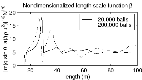
The length scale of the flow will also obey a differential equation depending on the Froude number

$$\frac{dL}{dt} = v \alpha(\mbox{Fr}),$$

where $\alpha(\mbox{Fr})$ is an unknown dimensionless function.

Different sized flows

Now we consider the equations applied to flows of $N$ balls. The mass of the flow $m = Nm_b$ and we define a dimensionless function $\beta$ such that $L = N^{1/3}r\beta$. $\beta$ will be of order 1 and independent of $N$ for non-degenerate flows. Equation  is then

$$\dot v = g \sin \theta - \rho \beta^2 r^2 v^2 N^{-1/3} m_b^{-1}$$

For steady state, $\dot v = 0$, it is immediately apparent that the velocity scales as

$$v = N^{-1/6}$$

. The middle of the track (the k-point) has constant angle and the front velocities of the flows are roughly constant. The excellent agreement is shown in fig. 3. The scaling constant is determined by least squares.

Figure 3: Front velocity at k-point

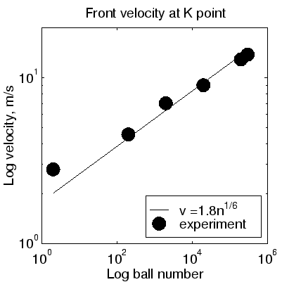
The success of this simple analysis is partly explained by the independence on $N$ of the relative density,

$$\frac{\rho L^3}{m}=\frac{\rho\beta}{m_b}$$

, and the Froude number,

$$\mbox{Fr}=\frac{Lg}{v^2}=\frac{\alpha}{\tilde v}$$

, where $\tilde v = v N^{-1/6}(rg)^{-1/2}$ is the non-dimensionalized velocity. The non-dimensionalized velocity is shown in fig. 4 for two flows of 20,000 and 200,000 balls. The initial surge out of the box is clearly seen after which the velocity decreases on the relatively flat slope. As the slope angle increases the flows accelerate to roughly the same (non-dimensionalized) velocity. The large variations in the velocities are due to inaccuracies in the measurement procedure.

Figure: non-dimensionalized velocity $\tilde v$

The data for front positions and velocities are limited and contains large errors so, at present, the data are too limited to quantatively analyze the length scale change functions $\alpha$ and $\beta$. However, fig  shows that after the initial surge it is at least plausible that $\beta$ is the same, roughly constant, function for both flows.

Figure 5: Length scale $\beta$

Structure of the flow

Air velocity data shows that air velocity increases over the length of the head ( $\approx 1\mbox{\,m}$) and that the air velocities are too low to overcome gravity -- vertical currents in excess of $7.5\mbox{\,m\,s}^{-1}$ would be necessary. Thus the air is not dragging the balls up in the head. On a smooth inelastic slope there are no forces to cause vertical ball motion, and indeed any such initial motion is rapidly damped out. This is confirmed by the two and three dimensional simulations. Table 1 shows the the velocity standard deviation in a flow calculated from the video camera data.

Table: Velocity standard deviation ( $\mbox{m\,s}^{-1}$) for a 300,000 ball flow

	head	body	tail
perpendicular	1.73	1.45	$<0.1$
down-slope	1.44	0.78	$<0.1$
cross-slope	0.72	0.56	$<0.1$

The interesting feature to notice here is the large downslope velocity deviation in the head compared to the body. This suggest that the height of the head, and the abrupt collapse of the height in the body can be explained as follows. The horizontal velocity of the air rapidly increases to the mean speed of the flow over the length of the head. The drag force accelerating the air strongly decelerates the balls leading to the high fluctuations in the down-slope velocity component. The balls collide and the horizontal velocity differences become vertical velocities thus causing the high head. In the body the drag of the air on the balls is very small since they are moving with similar velocities and there is much less internal motion so the height of the flow is much less. From another point of view, the drag force on the balls in the head increases the granular temperature and thus pressure in the head which can then support a large height of balls. Once the air has reached the mean speed the granular temperature (internal velocity variations) decrease and the height of the flow is reduced.

About this document ...

Modelling Ping-Pong Ball Avalanches

This document was generated using the LaTeX2HTML translator Version 99.2beta8 (1.42)

Copyright © 1993, 1994, 1995, 1996, Nikos Drakos, Computer Based Learning Unit, University of Leeds.
Copyright © 1997, 1998, 1999, Ross Moore, Mathematics Department, Macquarie University, Sydney.

The command line arguments were:
latex2html -image_type gif -split 0 miya_similarity.tex

The translation was initiated by Jim McElwaine on 2000-11-14